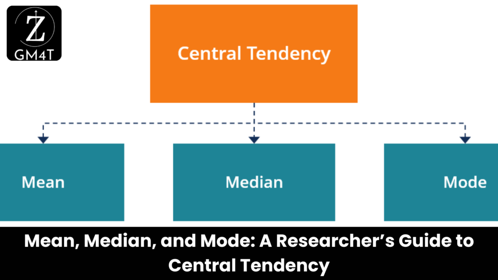
In data analysis, understanding central tendency—the point around which data values cluster—is crucial. The mean, median, and mode are the primary measures of central tendency. Each has its strengths and specific use cases, making them indispensable tools for summarizing data. Let’s explore these concepts with examples and practical applications.
1. Mean (Arithmetic Mean)
The mean is the most common measure of average. It’s calculated by summing all data values and dividing by the total number of observations.
Formula:
Example:
Suppose we have exam scores: 80, 85, 90, 95, and 100.
Key Features:
• Strengths: The mean considers all data points, making it ideal for statistical analysis.
• Limitations: It is sensitive to outliers. For example, adding a score of 300 to the dataset skews the mean upwards to 125, which no longer represents the majority of the data.
2. Median
The median is the middle value when observations are ordered from smallest to largest. For an even number of observations, the median is the average of the two middle values.
Example:
Dataset: 80, 85, 90, 95, 100
• Median: 90 (the middle value)
Dataset: 80, 85, 90, 95, 100, 300
• Median:
Key Features:
• Strengths: The median is robust against extreme values, making it a better choice when data contains outliers.
• Limitations: It doesn’t account for the magnitude of other observations, which may oversimplify some datasets.
3. Mode
The mode is the value that appears most frequently in a dataset. A dataset can be unimodal (one mode), bimodal (two modes), or multimodal (multiple modes).
Example:
Dataset: 80, 85, 90, 90, 95, 100
• Mode: 90 (appears twice)
Key Features:
• Strengths: Useful for categorical data where the most common category is of interest (e.g., the most frequently purchased product).
• Limitations: Rarely used for numerical data analysis and can be undefined if no value repeats.
Comparing Mean, Median, and Mode
The relationship between these measures depends on the data’s distribution:
• Symmetrical Distribution: Mean = Median = Mode
• Positively Skewed Distribution: Mean > Median > Mode
• Negatively Skewed Distribution: Mean < Median < Mode
Example:
In a positively skewed dataset (e.g., incomes where a few people earn significantly more):
• Mean might overestimate the central tendency.
• Median provides a more accurate reflection of typical values.
• Mode indicates the most common income bracket but misses nuances.
When to Use Which Measure?
1. Mean:
Best for datasets without outliers, as it incorporates all data points.
Use Case: Average exam scores, stock prices.
2. Median:
Preferred when outliers exist, as it reflects the central tendency without being skewed.
Use Case: Household income, property prices.
3. Mode:
Useful for identifying the most common category or value.
Use Case: Product preferences, survey responses.
Special Considerations: Skewed Data
In positively skewed data (e.g., incubation periods, income distributions), a geometric mean may be more appropriate than the arithmetic mean. The geometric mean is calculated as the -th root of the product of all values and reduces the impact of extreme values.
Final Thoughts
Understanding the differences between mean, median, and mode allows researchers to choose the most appropriate measure for their dataset. While the mean is often favored for its mathematical properties, the median and mode provide valuable insights, especially in datasets with outliers or skewed distributions.
Engage With Us: Which measure of central tendency do you rely on most in your research? Have you faced challenges with skewed data? Share your experiences in the comments below and stay tuned for more insights on statistical concepts!
